Lineshapes

All real measurements are the integral of the the true radiance \(I\) with what could be most accurately called the instrument response function. In one dimension, this looks like,

\[ S = \int I(x) R(x) dx,\]

where \(S\) is our measurement, \(I(x)\) is the radiance as a function of some dependent variable \(x\), and R(x) is the response function. The dependent variable is usually wavelength, wavenumber, or viewing angle. In skretrieval we refer to the response function as a lineshape since it is the “shape” that is observed if a delta function “line” is input to the instrument.

Usage

Let’s construct a Gaussian lineshape,

import numpy as np
import matplotlib.pyplot as plt
from skretrieval.core.lineshape import Gaussian

lineshape = Gaussian(fwhm=1.5)

The lineshape is agnostic about what the dependent variable is, in this case with setting fwhm=1.5 it is probably wavelength in nm, but the same lineshape class can be used for any dependent variable.

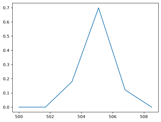
In skretrieval, a lineshape does not directly integrate over the radiance field, instead it provides the necessary quadrature weights to do the integration. We pass in the values of the dependent variable that we have samples of the radiance field at and it will return back the quadrature weights,

available_samples = np.arange(500, 510, 0.1)

weights = lineshape.integration_weights(mean=505, available_samples=available_samples)

plt.plot(available_samples, weights)

[<matplotlib.lines.Line2D at 0x750873514440>]

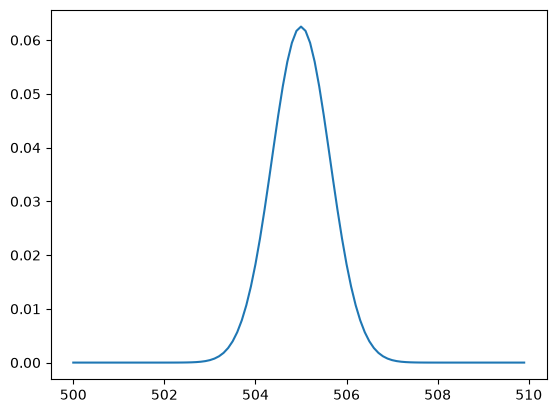
By default all lineshapes are normalized such that the sum of the weights is equal to 1.

Available Line Shapes

skretrieval.core.lineshape.DeltaFunction()	DeltaFunction line shape.
skretrieval.core.lineshape.Gaussian([fwhm, ...])	Gaussian line shape.
skretrieval.core.lineshape.Rectangle(width)	Rectangular line shape
skretrieval.core.lineshape.UserLineShape(...)	Line shape created from a user specified function

Technical Details about Lineshape Quadrature

Most of the lineshapes in skretrieval, and the main advantage in using these methods instead of your own lineshape, is that care has been taken to make the integration as accurate as possible. The Gaussian lineshape supports this through the optional mode= parameter. The best way to demonstrate how this works is through example.

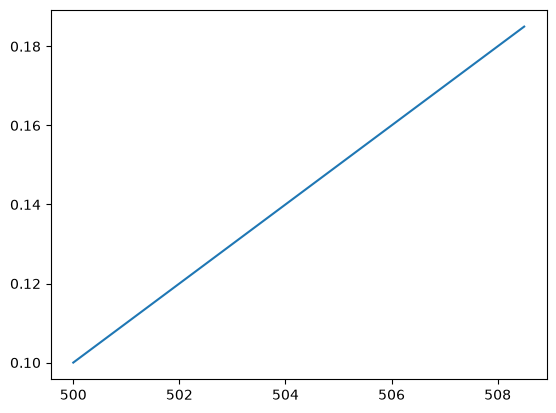
Let’s assume we have a radiance signal that varies linearly, but is coarsely sampled,

available_samples = np.arange(500, 510, 1.7)

radiance = 0.1 + (available_samples - 500) * 0.01

plt.plot(available_samples, radiance)

[<matplotlib.lines.Line2D at 0x750873301940>]

And let’s create a Gaussian lineshape and integrate the radiance

lineshape = Gaussian(fwhm=1.5, mode="constant")

weights = lineshape.integration_weights(mean=505, available_samples=available_samples)

plt.plot(available_samples, weights)

print(np.dot(radiance, weights))

0.1506077186029127

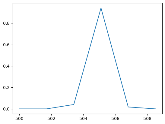
Clearly the Gaussian is very coarsely sampled, and we might be tempted to linearly interpolate the radiance to a higher resolution grid to obtain a more accurate answer

hires_grid = np.arange(500, 510, 0.01)

radiance_interp = np.interp(hires_grid, available_samples, radiance)

weights = lineshape.integration_weights(mean=505, available_samples=hires_grid)

plt.plot(hires_grid, weights)
print(np.dot(radiance_interp, weights))

0.15000000000000002

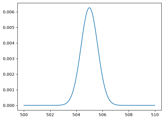
And we see that we get much closer to the true answer of 0.15. However, this interpolation could be onerous depending on the dimension of the problem. The power of skretrieval lineshapes is the mode="linear" parameter which will analytically compute the integration weights assuming linear interpolation of the radiances. For example, we can use this mode on the coarse resolution grid,

lineshape = Gaussian(fwhm=1.5, mode="linear")

weights = lineshape.integration_weights(mean=505, available_samples=available_samples)

plt.plot(available_samples, weights)

print(np.dot(radiance, weights))

0.1500146963112633

And we get very close to the analytic value while using the coarse resolution values.