Limb Scatter Polarized Aerosol Retrieval#
Here we set up a limb scatter aerosol retrieval similar to the previous example, except in this example we are both going to
Include a wavelength dependent Lambertian surface in the retrieval state vector
Modify the instrument to measure two orthogonal polarizations
We will start by setting up our observation. This is very similar to the previous example except in this case we are scaling the particle size separately from the extinction, only adjusting it in the 20-25 km altitude range.
import numpy as np
import sasktran2 as sk
import skretrieval as skr
import matplotlib.pyplot as plt


@skr.Retrieval.register_optical_property("stratospheric_aerosol")
def stratospheric_aerosol_optical_prop(*args, **kwargs):
    refrac = sk.mie.refractive.H2SO4()
    dist = sk.mie.distribution.LogNormalDistribution().freeze(mode_width=1.6)

    db = sk.database.MieDatabase(
        dist, refrac, np.array([469.0, 750.0]), median_radius=np.arange(10, 200, 10.0)
    )

    return db


# Measurement tangent altitudes
tan_alts = np.arange(10000, 45000, 1000)
altitude_grid = np.arange(0, 70000, 1000)

aerosol_scale = np.ones(len(altitude_grid))
aerosol_scale[20:25] = 1.5


sample_wavel = np.array([470.0, 745.0])

# Set up a simulated observation with our tangent altitudes, wavelengths
obs = skr.observation.SimulatedLimbObservation(
    cos_sza=0.6,
    relative_azimuth=0,
    observer_altitude=200000,
    reference_latitude=20,
    reference_longitude=20,
    tangent_altitudes=tan_alts,
    sample_wavelengths=sample_wavel,
    state_adjustment_factors={
        "stratospheric_aerosol": {
            "extinction_per_m": {"scale": 1.5},
            "median_radius": {"scale": aerosol_scale},
        }
    },  # Simulate with 1.5x the prior
)
Next we will do the standard retrieval, but will add in a spectrally varying albedo into the state vector.
# Set up the retrieval object
ret = skr.Retrieval(
    obs,
    minimizer="scipy",
    state_kwargs={
        "altitude_grid": altitude_grid,
        "aerosols": {
            "stratospheric_aerosol": {
                "type": "extinction_profile",
                "nominal_wavelength": 745,
                "retrieved_quantities": {
                    "extinction_per_m": {
                        "prior_influence": 1e-6,
                        "tikh_factor": 1e-1,
                        "min_value": 0,
                        "max_value": 1e-3,
                    },
                    "median_radius": {
                        "prior_influence": 1e0,
                        "tikh_factor": 1e-4,
                        "min_value": 10,
                        "max_value": 190,
                    },
                },
                "prior": {
                    "extinction_per_m": {"type": "testing"},
                    "median_radius": {"type": "constant", "value": 80.0},
                },
            },
        },
        "surface": {
            "lambertian_albedo": {
                "prior_influence": 0,
                "tikh_factor": 1e-4,
                "log_space": False,
                "wavelengths": sample_wavel,
                "initial_value": 0.3,
                "out_of_bounds_mode": "extend",
            },
        },
    },
    model_kwargs={
        "num_stokes": 3,
        "multiple_scatter_source": sk.MultipleScatterSource.DiscreteOrdinates,
        "num_streams": 8,
    },
)

results = ret.retrieve()
/home/docs/checkouts/readthedocs.org/user_builds/skretrieval/checkouts/stable/.pixi/envs/default/lib/python3.14/site-packages/scipy/optimize/_lsq/least_squares.py:905: UserWarning: Setting `xtol` below the machine epsilon (2.22e-16) effectively disables the corresponding termination condition.
  ftol, xtol, gtol = check_tolerance(ftol, xtol, gtol, method)
   Iteration     Total nfev        Cost      Cost reduction    Step norm     Optimality
       0              1         3.9747e+02                                    7.09e+09
1 2 5.1992e+00 3.92e+02 1.29e+02 1.56e+08
2 3 1.9928e-01 5.00e+00 6.24e+01 4.28e+07
3 4 2.0148e-02 1.79e-01 1.55e+01 2.48e+06
4 5 1.6287e-02 3.86e-03 4.20e+00 3.04e+05
5 9 1.6258e-02 2.88e-05 6.26e-01 5.78e+03
       6             10         1.6256e-02      2.11e-06       5.39e-01       2.50e+03
`ftol` termination condition is satisfied.
Function evaluations 10, initial cost 3.9747e+02, final cost 1.6256e-02, first-order optimality 2.50e+03.
And take a look at the resulting retrieved particle size
skr.plotting.plot_state(results, "stratospheric_aerosol_median_radius", show=False)
plt.subplot(1, 2, 1)
plt.plot(80 * aerosol_scale, altitude_grid, "k--")
plt.legend(["Retrieved", "Prior", "Truth"])
plt.show()
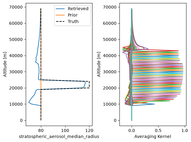
Note that there are some errors, we can also check the retrieved albedo
results["state"]["lambertian_albedo"]
<xarray.DataArray 'lambertian_albedo' (wavelengths_nm: 2)> Size: 16B
array([0.27409529, 0.305129  ])
Coordinates:
  * wavelengths_nm  (wavelengths_nm) float64 16B 470.0 745.0
And we see that it differs from the simulated value of 0.3.
Next we will repeat the calculation using a polarized instrument that measures (I+Q)/2 and (I-Q)/2 simultaneously.
# Set up the retrieval object
ret = skr.Retrieval(
    obs,
    minimizer="scipy",
    target_kwargs={"rescale_state_space": False},
    state_kwargs={
        "altitude_grid": altitude_grid,
        "aerosols": {
            "stratospheric_aerosol": {
                "type": "extinction_profile",
                "nominal_wavelength": 745,
                "retrieved_quantities": {
                    "extinction_per_m": {
                        "prior_influence": 1e-6,
                        "tikh_factor": 1e-1,
                        "min_value": 0,
                        "max_value": 1e-3,
                    },
                    "median_radius": {
                        "prior_influence": 1e0,
                        "tikh_factor": 1e-4,
                        "min_value": 10,
                        "max_value": 190,
                    },
                },
                "prior": {
                    "extinction_per_m": {"type": "testing"},
                    "median_radius": {"type": "constant", "value": 80.0},
                },
            },
        },
        "surface": {
            "lambertian_albedo": {
                "prior_influence": 0,
                "tikh_factor": 1e-4,
                "log_space": False,
                "wavelengths": sample_wavel,
                "initial_value": 0.3,
                "out_of_bounds_mode": "extend",
            },
        },
    },
    model_kwargs={
        "num_stokes": 3,
        "multiple_scatter_source": sk.MultipleScatterSource.DiscreteOrdinates,
        "num_streams": 8,
    },
    forward_model_cfg={
        "*": {
            "kwargs": {"stokes_sensitivities": {"vert": np.array([0.5, 0.5, 0, 0]), "horiz": np.array([0.5, -0.5, 0, 0])}}
        }
    },
)

results = ret.retrieve()

skr.plotting.plot_state(results, "stratospheric_aerosol_median_radius", show=False)
plt.subplot(1, 2, 1)
plt.plot(80 * aerosol_scale, altitude_grid, "k--")
plt.legend(["Retrieved", "Prior", "Truth"])
plt.show()
/home/docs/checkouts/readthedocs.org/user_builds/skretrieval/checkouts/stable/.pixi/envs/default/lib/python3.14/site-packages/scipy/optimize/_lsq/least_squares.py:905: UserWarning: Setting `xtol` below the machine epsilon (2.22e-16) effectively disables the corresponding termination condition.
  ftol, xtol, gtol = check_tolerance(ftol, xtol, gtol, method)
   Iteration     Total nfev        Cost      Cost reduction    Step norm     Optimality
       0              1         4.0072e+02                                    7.12e+09
1 2 5.7837e+00 3.95e+02 1.30e+02 6.32e+07
2 3 9.4585e-02 5.69e+00 6.29e+01 1.53e+07
3 4 9.7277e-03 8.49e-02 1.50e+01 5.97e+06
4 5 8.8562e-03 8.71e-04 2.50e+00 9.09e+04
5 6 8.8382e-03 1.81e-05 1.52e-01 2.60e+03
       6              7         8.8382e-03      1.68e-09       3.29e-03       1.48e+01
`ftol` termination condition is satisfied.
Function evaluations 7, initial cost 4.0072e+02, final cost 8.8382e-03, first-order optimality 1.48e+01.
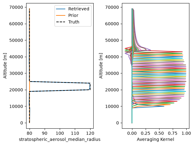
And we see that the results are better, with a more consistent surface albedo.
results["state"]["lambertian_albedo"]
<xarray.DataArray 'lambertian_albedo' (wavelengths_nm: 2)> Size: 16B
array([0.30034939, 0.30190275])
Coordinates:
  * wavelengths_nm  (wavelengths_nm) float64 16B 470.0 745.0
To enable polarization we added the lines
    forward_model_cfg={
        "*": {
            "kwargs": {"stokes_sensitivities": {"vert": np.array([0.5, 0.5, 0, 0]), "horiz": np.array([0.5, -0.5, 0, 0])}}
        }
    },
Which can be a bit confusing, so we can unpack what is going on. The first level of the dictionary "*" indicates that
this configuration applies to every measurement in our observation. This is important when our observation contains
multiple measurements that require separate forward models and we want to configure them separately.
The "kwargs" dictionary is the list of options that is passed to our forward model. In this case we are using
the default forward model, which uses the skretrieval.retrieval.forwardmodel.SpectrometerMixin instrument model. If we look at that
forward model we see it has a stokes_sensitivities input argument that we can set.