Limb and Nadir Synergistic Retrieval

In this example we combine limb scatter observations with nadir UV-VIS spectral observations to simultaneously retrieve a vertical ozone profile.

Let’s start by setting up a couple of things. Most of this setup follows the previous two examples on a limb scatter ozone retrieval and the nadir ozone retrieval examples, and you can skip over it if you are already familiar with it.

Show code cell source

Hide code cell source

import numpy as np
import skretrieval as skr

from skretrieval.core.lineshape import Gaussian

# Measurement tangent altitudes
tan_alts = np.arange(10000, 66000, 1000)

# Triplets
triplets = {
    "uv_1": {
        "wavelength": [302, 351],
        "weights": [1, -1],
        "altitude_range": [45000, 60000],
        "normalization_range": [60000, 65000],
    },
    "uv_2": {
        "wavelength": [312, 351],
        "weights": [1, -1],
        "altitude_range": [40000, 60000],
        "normalization_range": [60000, 65000],
    },
    "uv_3": {
        "wavelength": [322, 351],
        "weights": [1, -1],
        "altitude_range": [30000, 50000],
        "normalization_range": [60000, 65000],
    },
    "vis": {
        "wavelength": [525, 600, 675],
        "weights": [-0.5, 1, -0.5],
        "altitude_range": [0, 35000],
        "normalization_range": [35000, 40000],
    },
}

# Get the wavelengths required for the triplets
wavel = np.unique(np.concatenate([triplets[t]["wavelength"] for t in triplets])).astype(
    float
)

state_adjustment_factors = {"o3": 1.5}

# Set up a simulated observation with our tangent altitudes, wavelengths, and use 1.5x the initial guess for ozone
obs_limb = skr.observation.SimulatedLimbObservation(
    cos_sza=0.2,
    name="limb",
    relative_azimuth=0,
    observer_altitude=200000,
    reference_latitude=20,
    reference_longitude=20,
    tangent_altitudes=tan_alts,
    sample_wavelengths=wavel,
    state_adjustment_factors=state_adjustment_factors,  # Simulate with 1.5x the ozone of the prior
)

obs_nadir = skr.observation.SimulatedNadirObservation(
    cos_sza=0.2,
    name="nadir",
    cos_viewing_zenith=1.0,
    reference_latitude=20,
    reference_longitude=20,
    sample_wavelengths=np.arange(280, 800, 1.0),
    state_adjustment_factors=state_adjustment_factors,
)

state_kwargs = {
    "altitude_grid": np.arange(0, 70000, 1000),
    "absorbers": {
        "o3": {
            "prior_influence": 1e-1,
            "tikh_factor": 1e-1,
            "log_space": False,
            "min_value": 0,
            "max_value": 1,
            "prior": {"type": "mipas"},
        },
    },
    "surface": {
        "lambertian_albedo": {
            "prior_influence": 0,
            "tikh_factor": 1e-2,
            "log_space": False,
            "wavelengths": np.array([280, 360]),
            "initial_value": 0.5,
        }
    },
    "aerosols": {},
}

# Construct our measurement vectors
meas_vec_limb = {}
for name, t in triplets.items():
    meas_vec_limb[name] = skr.measvec.Triplet(
        t["wavelength"],
        t["weights"],
        t["altitude_range"],
        t["normalization_range"],
        apply_to_filter="limb",
    )

meas_vec_nadir = {}
meas_vec_nadir["nadir"] = skr.measvec.MeasurementVector(
    lambda l1, ctxt, **kwargs: skr.measvec.select(l1, **kwargs), apply_to_filter="nadir"
)

Above we have set up the

• simulated limb observation, and it’s associated measurement vector (discrete triplets)

• simulated nadir observation, and it’s associated measurement vector (the full spectrum)

• A few configuration options, including how to set up the state vector

Most of this is the same as the previous two examples, except note that we have added the apply_to_filter= option when constructing the respective measurement vectors. This ensures that each measurement vector will only apply to the observation that we want. We don’t want the full spectrum being used for the limb observation, and we don’t want to use triplets for the nadir retrieval.

First, let’s repeat what we have done before and just run the nadir retrieval.

ret = skr.Retrieval(
    obs_nadir,
    measvec=meas_vec_nadir,
    minimizer="rodgers",
    target_kwargs={"rescale_state_space": True},
    state_kwargs=state_kwargs,
)

results = ret.retrieve()
skr.plotting.plot_state(results, "o3_vmr", show=True)

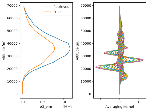
And then let’s repeat the limb scatter retrieval,

ret = skr.Retrieval(
    obs_limb,
    measvec=meas_vec_limb,
    minimizer="rodgers",
    target_kwargs={"rescale_state_space": True},
    state_kwargs=state_kwargs,
)

results = ret.retrieve()
skr.plotting.plot_state(results, "o3_vmr", show=True)

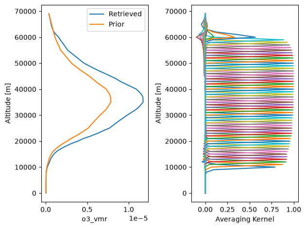
Comparing both retrieval averaging kernels we see that the nadir retrieval has very wide averaging kernels, but has some sensitivity into the troposphere. The limb scatter averaging kernel has very narrow averaging kernels, but has zero sensitivity into the troposphere.

We can now perform a joint retrieval. Combining the measurements is as simple as adding the observations together, and merging the measurement vectors.

ret = skr.Retrieval(
    obs_limb + obs_nadir,
    measvec={**meas_vec_limb, **meas_vec_nadir},
    minimizer="rodgers",
    target_kwargs={"rescale_state_space": True},
    state_kwargs=state_kwargs,
)

results = ret.retrieve()
skr.plotting.plot_state(results, "o3_vmr", show=True)

/home/docs/checkouts/readthedocs.org/user_builds/skretrieval/checkouts/stable/src/skretrieval/retrieval/target/__init__.py:42: RuntimeWarning: invalid value encountered in log
  internal_x[both_bounds] = np.log(
/home/docs/checkouts/readthedocs.org/user_builds/skretrieval/checkouts/stable/src/skretrieval/retrieval/target/__init__.py:42: RuntimeWarning: invalid value encountered in log
  internal_x[both_bounds] = np.log(

---------------------------------------------------------------------------
ValueError                                Traceback (most recent call last)
Cell In[4], line 9
      5     target_kwargs={"rescale_state_space": True},
      6     state_kwargs=state_kwargs,
      7 )
      8 
----> 9 results = ret.retrieve()
     10 skr.plotting.plot_state(results, "o3_vmr", show=True)

File ~/checkouts/readthedocs.org/user_builds/skretrieval/checkouts/stable/src/skretrieval/retrieval/processing.py:381, in Retrieval.retrieve(self, enabled_state_elements, enabled_measurement_vectors)
    377             val.enabled = False
    379 self._target.update_state_slices()
--> 381 min_results = minimizer.retrieve(
    382     self._obs_l1, self._forward_model, self._target
    383 )
    385 # Reset the enabled flag
    386 for _, val in self._state_vector.sv.items():

File ~/checkouts/readthedocs.org/user_builds/skretrieval/checkouts/stable/src/skretrieval/retrieval/rodgers.py:321, in Rodgers.retrieve(self, measurement_l1, forward_model, retrieval_target)
    319 if np.isnan(chi_sq) or np.isinf(chi_sq):
    320     msg = "chi_sq is infinite or nan"
--> 321     raise ValueError(msg)
    323 chi_sq_only_meas_linear /= len(y_meas)
    324 chi_sq_linear /= len(y_meas)

ValueError: chi_sq is infinite or nan

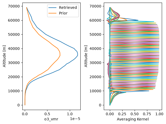
We can see that the joint averaging kernel retains the high vertical resolution in the stratosphere from the limb scatter retrieval, and has improved tropospheric sensitivity relative to just the nadir retrieval.