Quick Start

The atmospheric inverse problem at it’s core is solving the problem given a set of measurements \(\mathbf{y}\) which depend on atmospheric state parameters \(\mathbf{x}\), what is our best estimate of \(\mathbf{x}\). We assume that we have a “Forward Model” that is capable of taking \(\mathbf{x}\) as input, and producing simulated observations. The atmospheric retrieval problem is the inverse of this, going from measurements to atmospheric state.

As a first introduction to skretrieval, we are going to set up a simulated retrieval where a Nadir viewing instrument is measuring backscattered radiation across the UV-VIS spectrum and our goal is to estimate the observed ozone concentration. We start by creating a skretrieval.observation.Observation object which defines the measurements,

import skretrieval as skr
import numpy as np

observation = skr.observation.SimulatedNadirObservation(cos_sza=0.6,
                                                        cos_viewing_zenith=1.0,
                                                        reference_latitude=20,
                                                        reference_longitude=0,
                                                        sample_wavelengths=np.arange(280, 800, 0.5),
                                                        state_adjustment_factors={"o3": 1.5})

In this case we have created a special kind of observation, a “Simulated Observation”, which means that we are going to use our forward model to simulate measurements rather than using measurements from a real instrument. Since our observation is simulated, we have to specify some parameters about where we are looking, what we are measuring, etc. We also specify state_adjustment_factors which are some options to change the atmospheric state in our simulation, will come back to that later.

Then we can set up the main retrieval class

ret = skr.Retrieval(observation,
                    state_kwargs={
                        "altitude_grid": np.arange(0, 70000, 1000),
                        "absorbers": {
                        "o3": {
                            "prior_influence": 1e-1,
                            "tikh_factor": 1e-1,
                            "log_space": False,
                            "min_value": 0,
                            "max_value": 1,
                        },
                      },
                    }
                    )

The main thing we had to specify is state_kwargs. This defines our atmospheric state \(\mathbf{x}\), as well as any priors we attach to it. In this case, the quantities that we are retrieving is just ozone, and note that we have given it the name “o3” which matches what we had provided in state_adjustment_factors earlier. This means that our simulation is going to use 1.5x the amount of ozone as our initial guess.

Then we can perform the retrieval

results = ret.retrieve()

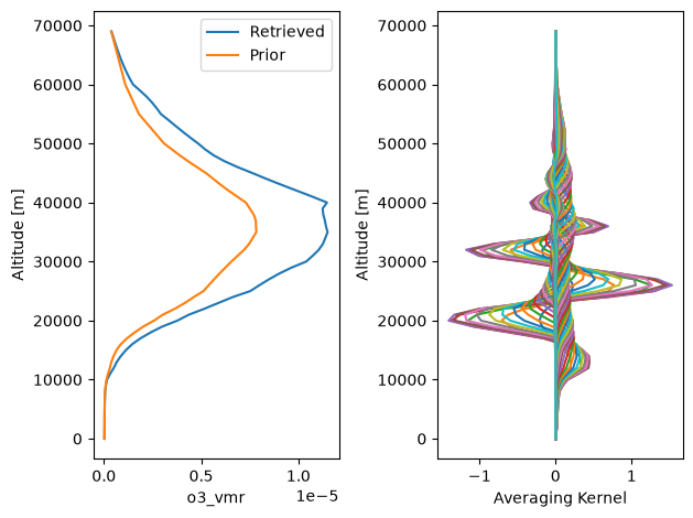
And we can look at some of the results

skr.plotting.plot_state(results, "o3_vmr")

skretrieval provides default settings for most aspects of the retrieval including

• Setting up how the observations are modelled (the forward model)

• Choosing and transforming which measurements to include in the retrieval (the measurement vector)

• How ancillary information is included in the atmosphere

• How the atmospheric state is constructed from the configuration parameters

All of these things can be overrided by the user, and more details on how this is done is found in the user’s guide.